How the Theory of Constraints finds the one resource that limits throughput: five focusing steps, bottleneck analysis and Drum-Buffer-Rope.
TL;DR: The Theory of Constraints (TOC) holds that every system has one constraint that limits its throughput, so improving anything else adds little. In manufacturing the constraint is often the slowest or most overloaded resource, which machine monitoring software makes visible. TOC finds it, gets more from it, aligns everything else to it, and adds capacity only if that is not enough.
Key Takeaways
- One constraint sets throughput: An hour lost there is an hour lost for the whole plant.
- Five focusing steps: Identify, exploit, subordinate, elevate and repeat.
- Busy is not better: Maximizing every machine’s utilization can lower throughput by flooding the constraint with WIP.
- Data shows where it sits: Utilization, cycle time, starvation, blocking and downtime data show where the constraint sits and when it moves.
Bottleneck Analysis: Finding the Constraint with Data
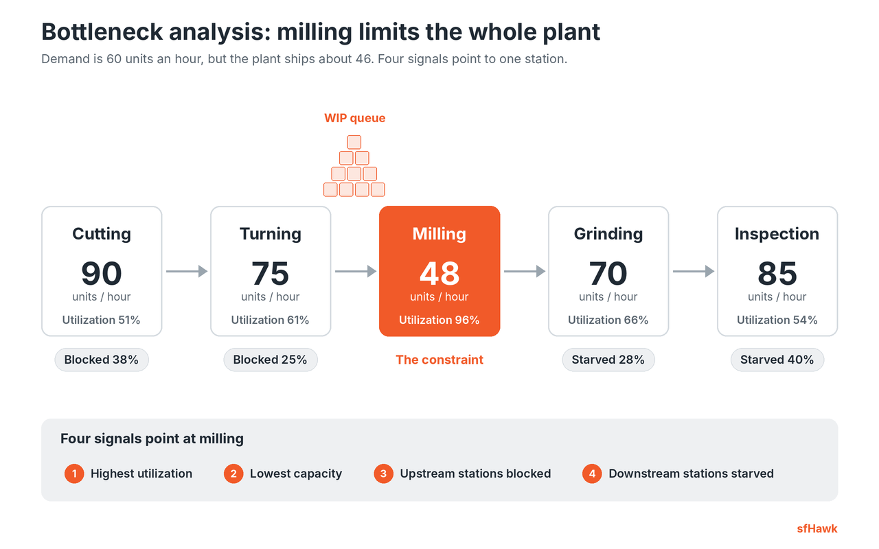
Our example is a fictional machine shop making valve bodies through five stations. Demand is 60 units an hour, but the plant ships about 46. Four weeks of machine data from production monitoring software show:
| Station | Capacity per hour | Utilization | Blocked | Starved |
|---|---|---|---|---|
| Cutting | 90 | 51% | 38% | 0% |
| Turning | 75 | 61% | 25% | 3% |
| Milling | 48 | 96% | 0% | 2% |
| Grinding | 70 | 66% | 0% | 28% |
| Inspection | 85 | 54% | 0% | 40% |
Four signals point at milling: the highest utilization, the lowest capacity, blocked stations upstream because its queue is full, and starved stations downstream waiting for its output. Check all four, since the busiest-looking station is not always the constraint. OEE monitoring then breaks the constraint’s losses into availability, performance and quality, so you know where to start.
The Theory of Constraints Five Focusing Steps, Applied
- Identify: Milling, at 48 units an hour with a queue in front of it, limits the plant.
- Exploit: Get more from milling before spending money. Operators are relieved during breaks, the next job is set up offline, and first-piece approval moves ahead of milling so scrap is not machined. Effective output rises from 46 to 52 units an hour.
- Subordinate: Every other station works to milling’s pace. Cutting and turning stop running ahead of it, so their blocked time is no longer treated as a loss. It is the cost of protecting the constraint.
- Elevate: Demand is still 60. A new fixture shortens the milling cycle and one job family moves to a second machine, lifting capacity to 66 units an hour. The plant now ships 60.
- Repeat: Grinding at 70 units an hour is next in line, and the market now sets the limit. The constraint will move as demand and product mix change.
Bottleneck, Constraint and Capacity Issue
| Term | Meaning | In the example |
|---|---|---|
| Constraint | Whatever limits the system’s throughput. It can be a machine, a policy, supply or the market | Milling now, perhaps the market later |
| Bottleneck | A resource with less capacity than the demand placed on it | Milling at 48 against 60 |
| Capacity issue | A local problem such as frequent stops, at a resource that still has more capacity than the constraint | Grinding at 70 with frequent stops |
A capacity issue becomes a capacity constraint only if that resource falls below the current constraint. Until then, fixing it does not raise plant output.
Drum-Buffer-Rope
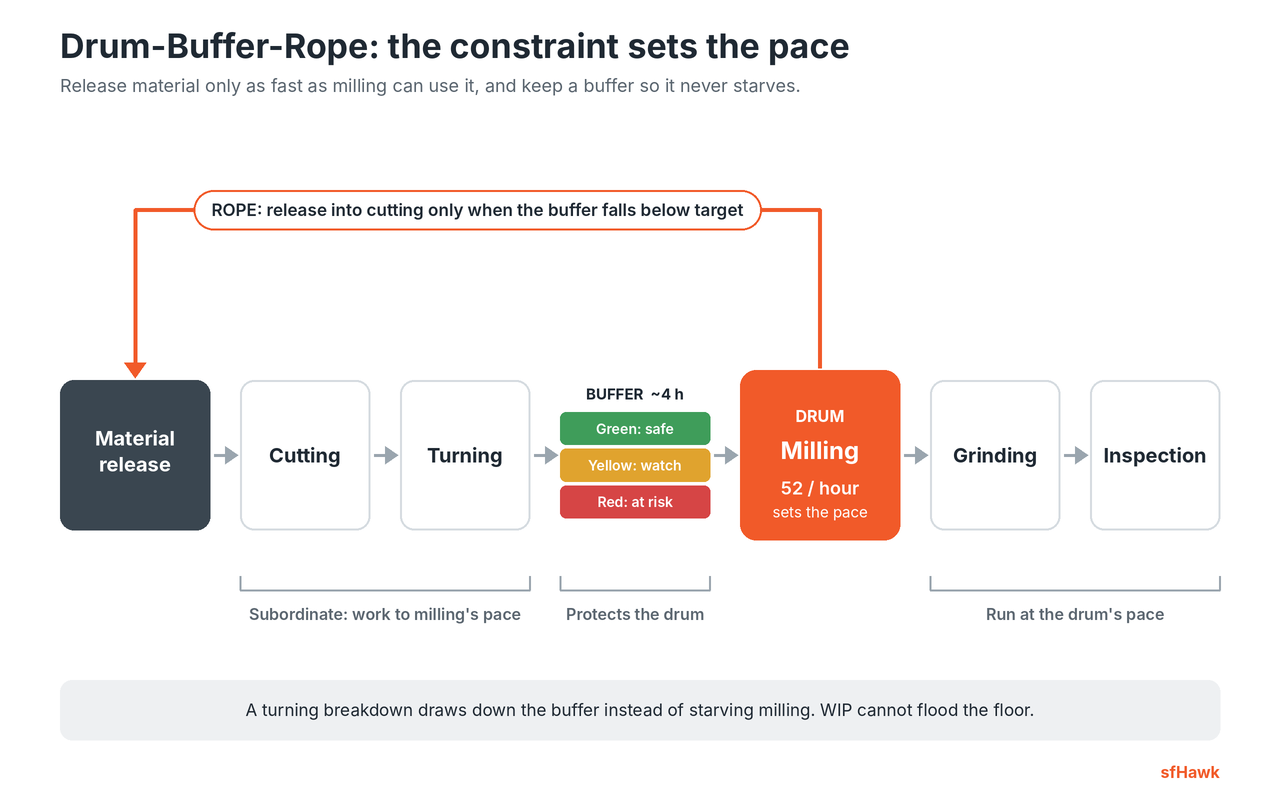
Drum-Buffer-Rope (DBR) is the scheduling method that keeps the other steps in place:
- Drum: Milling’s schedule sets the pace of the plant, 52 units an hour after step two.
- Buffer: About four hours of work waits in front of milling, so a turning breakdown does not starve it. Buffer status is tracked in green, yellow and red zones, and red means the constraint is at risk.
- Rope: Material is released into cutting only when the buffer falls below target, so WIP cannot flood the floor.
“Everyone wants their own machine to look busy. A busy machine feeding a queue is just making inventory, and the plant ships exactly what the constraint ships.”
[Name], [Designation], [Company]
Measuring Whether the Change Worked
An hour lost at the constraint is lost for the whole plant, while an hour saved elsewhere adds nothing to output. That makes measurement essential. sfHawk records running, idle and stopped time, cycle time, output and downtime reasons for each connected machine. Blocked and starved periods appear as waiting time when those reasons are coded, such as waiting for material.
Teams can confirm the constraint from data, track its throughput each shift after every change, and see the day it moves to another station. Our posts on assembly line bottlenecks and hidden capacity go deeper.
Frequently Asked Questions
What is the difference between TOC and lean?
Lean removes waste across the whole value stream. TOC starts by finding the single constraint and focuses improvement there. They work well together: TOC says where to focus first, and lean supplies the tools to remove waste at that point.
Can bottlenecks move?
Yes. They move after you elevate the constraint, when product mix changes and different parts load different machines, after breakdowns, and when shifts or staffing change. That is why the last step is to repeat, and why daily data matters.
References: Goldratt and Cox, The Goal (1984); Goldratt, Theory of Constraints (1990); Schragenheim and Dettmer, Manufacturing at Warp Speed (2000).
Related Reading
Finding the constraint starts with honest run, stop and wait time for every machine. See how machine monitoring software captures it by station, and how production monitoring software tracks constraint output shift by shift. For more, read Assembly Line Monitoring and Industry 4.0: Finding the Bottleneck Station, Hidden Capacity: How Manufacturers Increase Output Without Buying New Machines, and Line Balancing in Manufacturing.
Get Started Today! Book a call with sfHawk | Email: inquiry@sfhawk.com | Phone: +91 91120 98351 | Website: www.sfhawk.com